You should have enough information about the google sheet to make the google sheet most productive. So, I've collected here the most important Formula Tips & Tricks of google sheet you need, in your learning path. And then see who's stopping you from being a master in google worksheet.
So, let's move straight to Google sheet tutorial - Tips & Formula
After completion of google sheet tutorial, YOU are able to:
1. Use of F2 function key in google sheet
2. Use of Enter key in google spreadsheet
3. Use of Escape Key in google sheet
4. Use of F1 key in google sheet
5. Use of Tab key in google spreadsheet
6. How to Translate Languages With Google Sheets
7. How to create QR codes with Google Sheets formula
8. Google Sheets Functions – ISEMAIL()
10. How to Change Text Case in Google Sheets ?
11. How to Remove Extra Spaces or Additional Spaces From Data in Google Spreadsheets
13. How to Use ISURL Function in Google Sheets ?
14. How to Insert an Image in a Cell in Google Sheets
15. How to Protect Sheets & Lock Cells in Google Sheets
Use of F2 function key in google sheet:
To Edit selected cell, just select the cell and click F2 and you will be able to edit in that cell.
Use of Enter key in google spreadsheet:
To enter or exit formula or to enter or exit edit view with saving changes you have made.
Use of Escape Key in google sheet:
To Exit a Formula, or to click out of the edit view / formula view.
But keep in mind when using Escape Key that any changes made you already are discarded when you press the Escape key.
Use of F1 key in google sheet:
To turn on Formula Help.Formula Help would be helpful to recognize and efficiently use the google sheet formula.
Use of Tab key in google spreadsheet:
Tab key is used to Auto Complete Function Name in google spreadsheet. When you type function in cell, formula help will appear. If formula help does not show then press F1 key to turn on formula help.And Then press the Tab key to auto complete the function name which is highlighted into formula help dropdown list.
How to Translate Languages With Google Sheets - From one language to other language using GOOGLETRANSLATE google sheet function
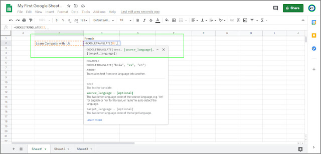
You can translate one language to other using GOOGLETRANSLATE function in google sheet.
Syntax:=GOOGLETRANSLATE(text, [source_language], [target_language])
Example of GOOGLETRANSLATE:
=GOOGLETRANSLATE(B2,"en","fr")
=GOOGLETRANSLATE(B2,"en","hi")
=GOOGLETRANSLATE(B2,"en","gu")
=GOOGLETRANSLATE(B2,"en","hi")
=GOOGLETRANSLATE(B2,"en","gu")
- For other language code that you can use in google translate function: Languages Codes click here
You can create QR Codes using Google sheet:
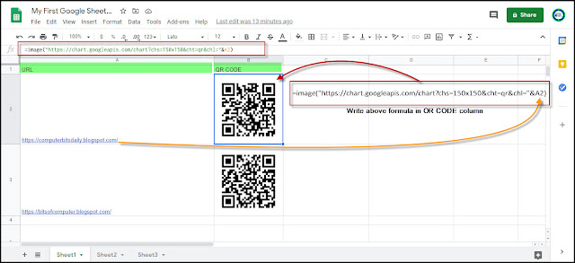
- To Create QR CODE , you need to create a two column in google sheet, and label it as 'URL' and 'QR Code' as shown in the image below.
- Now in the first column (column address is A2) simply type the text or url for which one you want to generate the QR code.
- Here I have written “ https://computerbitsdaily.blogspot.com/ “ In URL column.
- After that, in the OR Code column, copy and paste this formula. Please refer to the picture below for better understanding.=image("https://chart.googleapis.com/chart?chs=150x150&cht=qr&chl="&A2)
- And, QR code will appeared.
Let’s understand above formula:
In given formula (=image("https://chart.googleapis.com/chart?chs=150x150&cht=qr&chl="&A2)
) ‘A2’ at the end of the formula is the cell address that contains the URL or Text data, that you want to create the QR code for.
The same way, when you want to generate QR code for the text or URL in A3 cell then, simply write A3 in formula as shown below.
=image("https://chart.googleapis.com/chart?chs=150x150&cht=qr&chl="&A3)
- You can copy and paste this generated QR code.
Check email address properly formatted or not using google sheet function:
To check collected email address or entered email address is properly formatted or not in google sheet, you can simply use =ISEMAIL(“EMAIL ADDRESS/CELL ADDRESS CONATAINING EMAIL ADDRESS”) formula in google sheet.Sheets will return “TRUE” for properly formatted email address and “FALSE” for not formatted properly.
Example of ISEMAIL() in google worksheet:
=ISEMAIL("bitsofcomputer@gmail.com")=ISEMAIL(“A2”)
Change Case OF any string or text in google sheet: You can do this task using following google sheet function.
=UPPER(“Text” or Cell address which contain text) :
This function transforms the text to a Upper case in google sheet.
=LOWER((“Text” or Cell address which contain text) :
This function transforms the text to a Lower case in google sheet.
=PROPER((“Text” or Cell address which contain text):
This function transforms the text to a Proper case in google sheet.
How to Remove Extra Spaces or Additional Spaces From Data in Google Spreadsheets:
You can remove extra space using TRIM() function or Find and Replace Command in google sheet.Using Trim Function:
The TRIM function can also be used to eliminate those extra spaces.
Syntax:
TRIM(Text or Cell address)
Example:
=Trim(“Computer Bit : The Best Place to Learn computer)
Out Put of Trim function: This function will remove all extra space from taken string into function and result will be “Computer Bit : The Best Place to Learn computer”
Ctrl + H or simply go to Edit --> Find and Replace.
Steps:
- Open the google sheet tab where you want to remove extra space.
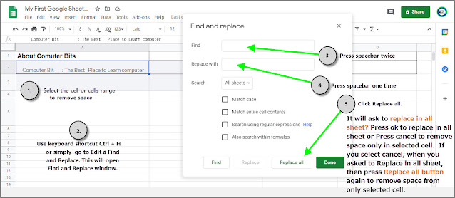
- Use keyboard shortcut Ctrl + H or simply go to Edit --> Find and Replace. This will open Find and Replace window.
- In this Find and Replace window, in Find textbox press spacebar twice and in Replace with text box press spacebar once.
- Now click Replace all, it will ask to replace in all sheet?
If you want Replace in all sheet, then simply press ok or press cancel to remove space only in selected cell. If you select cancel, when you asked Replace in all sheet then press Replace all again to remove space from only selected cell.
- And last task is to press Done button.
Google Sheets =ISURL() Function:
Syntax:
=ISURL(value)
The purpose of this google sheet function is to check valid URLs. The ISURL() formula will return TRUE or FALSE. If the ISURL() formula returns a TRUE, then that the provided ‘value’ is a valid URL. If the ISURL() formula returns a FALSE, then that provided value is not valid URL.
Add an image to a google spreadsheet using IMAGE():
Syntax of the IMAGE() function:
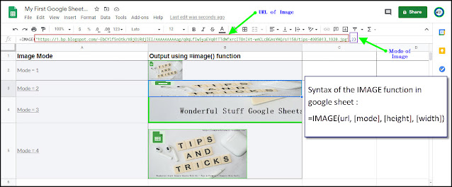
=IMAGE(url, [mode], [height], [width])
url: The link of the image.
mode: The mode is 1 by default.
-- Size 1 to fit inside the cell. Don’t give value for height and width.
-- Size 2 compresses or stretches picture to fit in the cell. Don’t give value for height and width.
-- Size 3 will crop the image to fits in the cell. Don’t give value for height and width.
-- Size 4 allows the user to select the size (height/width) of the image.
height : To set height of Image. To avail height, make sure your mode is 4.
width: To set width of Image. To avail height, make sure your mode is 4.
How to Protect Sheets & Lock Cells in Google Sheets:
Steps to lock a cell in Google Sheets (Only you can change):
-- Right-click on the cell that you want to lock
-- Click on Protect range option.
-- Click on Protect range option.
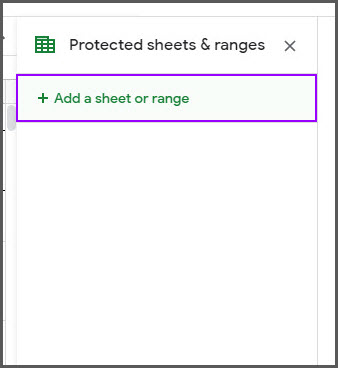
-- Now, click on Add a sheet or Range. On clicking this, it will ask to enter “Description (Optional)” and Range.
-- Enter description and range of cell or address of single cell to make it protected.
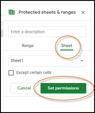
--And Press Set Permission.
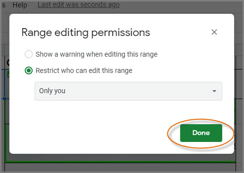
-- On clicking Set Permission, it will open range editing permission. Simply Press Done.
-- If you want to give access of sheet, to some other user the select custom in this window.
-- That’s it you successfully lock cell or range.
-- You can protect entire sheet by selecting sheet option in protected sheets and ranges window in google sheet. See in image for better understanding.
Hope you will find this stuff useful. What other google sheet tips or formula can you add to this list that I may have not mentioned? Leave in the comment section. If you enjoyed this google sheet tutorial, please share it with all your friends and loved one!
Unlock Learning ✌ | Keep Sharing | Stay Safe.😷










0 Comments